SVP64 REMAP Worked Example: Matrix Multiply
Links
- Online matrix calculator
- remap
- https://bugs.libre-soc.org/show_bug.cgi?id=701
- video https://m.youtube.com/watch?v=BbhOA8ULKt4 slides https://ftp.libre-soc.org/openpower_2021.pdf
- setvl instruction: setvl
- standalone-executable REMAP python function based on generator-yielding (shows how indices are generated): remapyield.py
One of the most powerful and versatile modes of the REMAP engine (a part of the SVP64 feature set) is the ability to perform matrix multiplication with all elements within a scalar register file.
This is done by converting the index used to iterate over the operand and result matrices to the actual index inside the scalar register file.
Worked example - manual (conventional method)
The matrix multiply looks like this:
mat_X * mat_Y = mat_Z
When multiplying non-square matrices (rows != columns), to determine the
dimension of the result when matrix X has a rows and b columns and matrix
Y has b rows and c columns:
X_axb * Y_bxc = Z_axc
The result matrix will have number of rows of the first matrix, and number of columns of the second matrix.
For this example, the following values will be used for the operand matrices X and Y, result Z shown for completeness.
    X =| 1 2 3 |  Y =  |  6  7 |  Z = |  52  58 |
       | 3 4 5 |       |  8  9 |      | 100 112 |
                       | 10 11 |
Matrix X has 2 rows, 3 columns (2x3), and matrix Y has 3 rows, 2 columns.
To determine the final dimensions of the resultant matrix Z, take the number of rows from matrix X (2) and number of columns from matrix Y (2).
The method usually taught in linear algebra course to students is the following (outer product):
- Start with the first row of the first matrix, and first column of the second matrix.
- Multiply each element in the row by each element in the column, and sum with the current value of the result matrix element (multiply-add-accumulate). Store result in the row matching first operand row and column matching second operand column.
- Move to the next column of the second matrix, and next column of the result matrix. If there are no more columns in the second matrix, go back to first column (second matrix), and move to next row (first and result matrices). If there are no more rows left, result matrix has been fully computed.
- Repeat step 2.
This for-loop uses the indices as shown above
for i in range(0, mat_X_num_rows):
    for k in range(0, mat_Y_num_cols):
        for j in range(0, mat_X_num_cols): # or mat_Y_num_rows
            mat_Z[i][k] += mat_X[i][j] * mat_Y[j][k]
Calculations:
    | 1 2 3 |   |  6  7 | = | (1*6 + 2*8 + 3*10) (1*7 + 2*9 3*11) |
    | 3 4 5 | * |  8  9 |   | (3*6 + 4*8 + 5*10) (3*7 + 4*9 5*11) |
                | 10 11 |

    | 1 2 3 |   |  6  7 | = | ( 6 + 16 + 30) ( 7 + 18 + 33) |
    | 3 4 5 | * |  8  9 |   | (18 + 32 + 50) (21 + 36 + 55) |
                | 10 11 |

    | 1 2 3 |   |  6  7 | = |  52  58 |
    | 3 4 5 | * |  8  9 |   | 100 112 |
                | 10 11 |
For the algorithm, assign indices to matrices as follows:
    Index | 0 1 2 3 4 5 |
    Mat X | 1 2 3 3 4 5 |

    Index | 0  1  2  3  4  5 |
    Mat Y | 6  7  8  9 10 11 |

    Index |   0   1   2   3 |
    Mat Z |  52  58 100 112 |
(Start with the first row, then assign index left-to-right, top-to-bottom.)
Index list:
    | Mat X | Mat Y | Mat Z |
    |   0   |   0   |   0   |
    |   1   |   2   |   0   |
    |   2   |   4   |   0   |
    |   0   |   1   |   1   |
    |   1   |   3   |   1   |
    |   2   |   5   |   1   |
    |   3   |   0   |   2   |
    |   4   |   2   |   2   |
    |   5   |   4   |   2   |
    |   3   |   1   |   3   |
    |   4   |   3   |   3   |
    |   5   |   5   |   3   |
Worked example broken down into individual multiply-add accumulates:
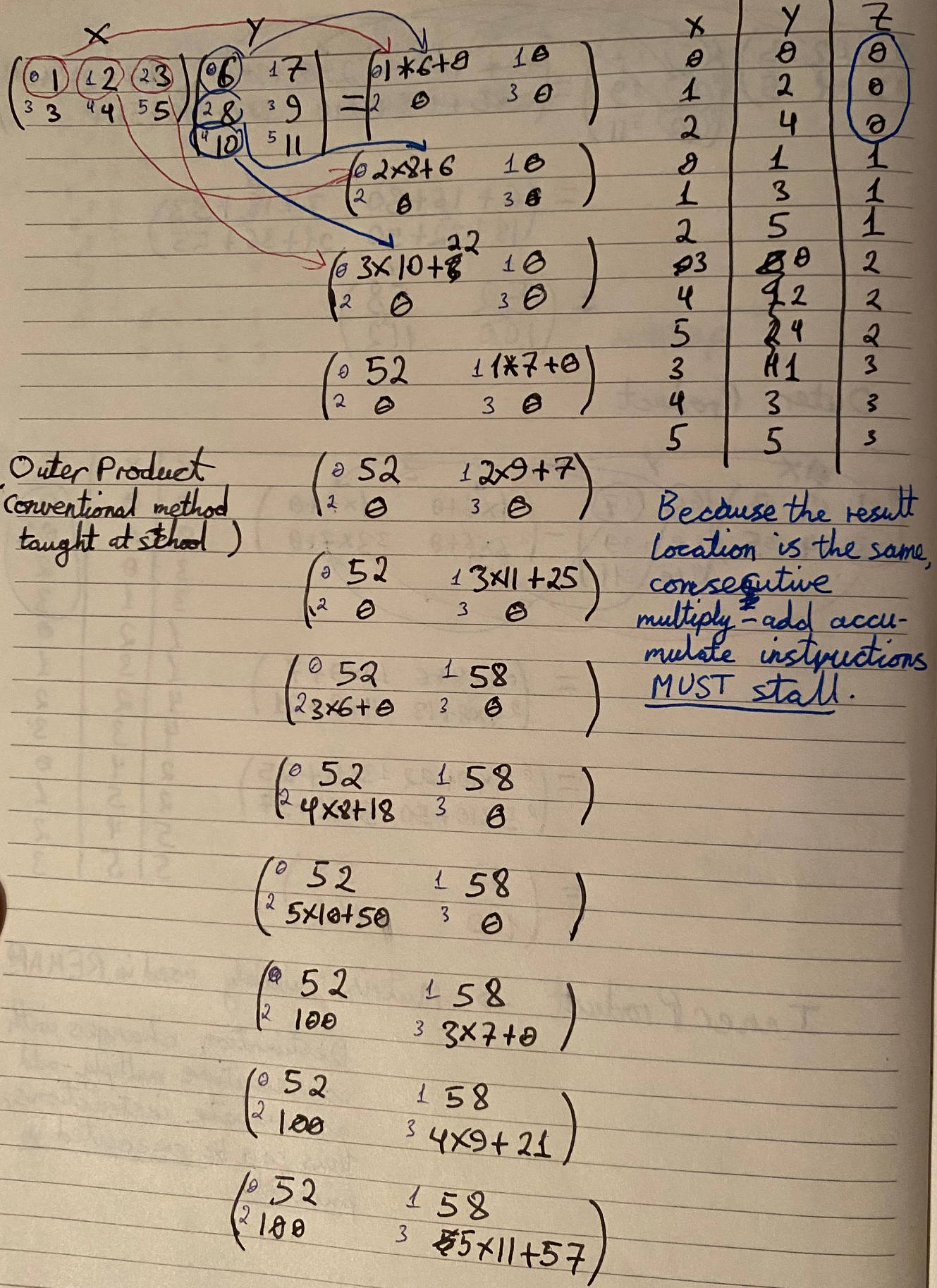
The issue with this algorithm is that the result matrix element is the same for three consecutive operations, and where each element is stored in CPU registers, the same register will be written to three times and thus causing consistent stalling.
Inner Product
A slight modification to the order of the loops in the algorithm massively reduces the chance of read-after-write hazards, as the result matrix element (and thus register) changes with every multiply-add operation.
The code:
for i in range(mat_X_num_rows):
    for j in range(0, mat_X_num_cols): # or mat_Y_num_rows
        for k in range(0, mat_Y_num_cols):
            mat_Z[i][k] += mat_X[i][j] * mat_Y[j][k]
Index list:
    | Mat X | Mat Y | Mat Z |
    |   0   |   0   |   0   |
    |   0   |   1   |   1   |
    |   3   |   0   |   2   |
    |   3   |   1   |   3   |
    |   1   |   2   |   0   |
    |   1   |   3   |   1   |
    |   4   |   2   |   2   |
    |   4   |   3   |   3   |
    |   2   |   4   |   0   |
    |   2   |   5   |   1   |
    |   5   |   4   |   2   |
    |   5   |   5   |   3   |
Worked example for inner product:
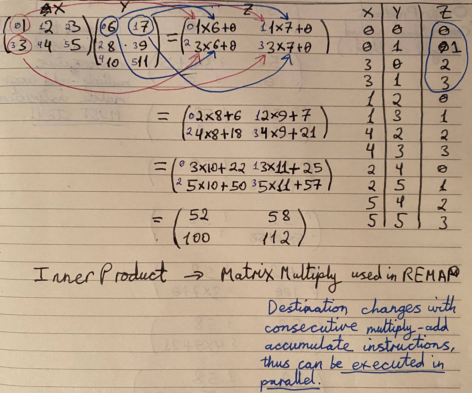
The index for the result matrix changes with every operation, and thus the consecutive multiply-add instruction doesn't depend on the previous write register.
Outer and inner product indices side-by-side:
    |   Outer Product       |   Inner Product       |
    | Mat X | Mat Y | Mat Z | Mat X | Mat Y | Mat Z |
    |   0   |   0   |   0   |   0   |   0   |   0   |
    |   1   |   2   |   0   |   0   |   1   |   1   |
    |   2   |   4   |   0   |   3   |   0   |   2   |
    |   0   |   1   |   1   |   3   |   1   |   3   |
    |   1   |   3   |   1   |   1   |   2   |   0   |
    |   2   |   5   |   1   |   1   |   3   |   1   |
    |   3   |   0   |   2   |   4   |   2   |   2   |
    |   4   |   2   |   2   |   4   |   3   |   3   |
    |   5   |   4   |   2   |   2   |   4   |   0   |
    |   3   |   1   |   3   |   2   |   5   |   1   |
    |   4   |   3   |   3   |   5   |   4   |   2   |
    |   5   |   5   |   3   |   5   |   5   |   3   |
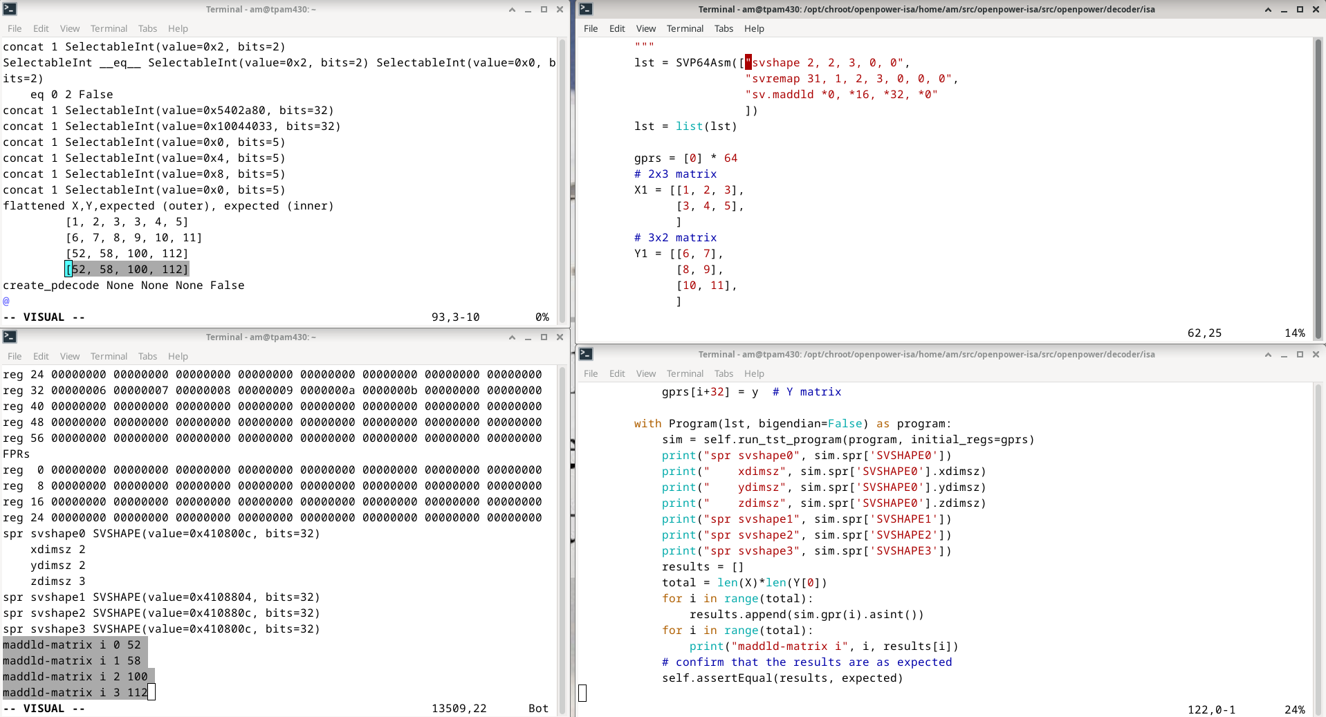
SVP64 instructions implementing matrix multiply
- SVP64 assembler example: unit test
- svremap and svshape instructions defined in: [[sv/rfc/ls009]
- Multiple-Add Low Doubleword instruction pseudo-code (Power ISA 3.0C Book I, section 3.3.9): fixedarith
    svshape 2, 2, 3, 0, 0
    svremap 15, 1, 2, 3, 0, 0, 0
    sv.maddld *0, *16, *32, *0
As you can see, only three instructions are required to perform arbitrary matrix multiplication, with non-power-of-2 matrices!
The reason why the main part of matrix multiplication is so simple is down to three reasons:
- a RISC ISA is used as the fundamental basis, with powerful and simple instructions (Power ISA)
- Simple-V REMAP indexing system - generates index schedules for a range of problems: matrix multiply, FFT, DCT, programmer-defined, etc.
- Simple-V SVP64 looping system based on instruction prefixing which turns any scalar instruction into a vector one. Can follow consecutive element indexing, or REMAP schedule indexing.
Additionally, if instead of matrix multiplication, a different operation is
required (say, to perform logical operations on rows/cols), the third
instruction - maddld - can be substituted for a different operation. This is
beyond the scope of this guide, however it should be clear that using
fmadds instead would perform a FP32 matrix multiply, just by replacing maddld.
svshape
The svshape instruction is a convenient way to set up the SVSHAPE Special
Purpose Registers (SPRs), which were added alongside the SVP64 looping
system for complex element indexing. Without having "Re-shaping" SPRs,
only the most basic, consecuting indexing of register elements (0,1,2,3...)
would be possible.
The REMAP system has 16 modes, all of which are accessible through the
svshape instruction. However for the purpose of this guide, only SVrm=0
(Matrix Multiply, Inner Product) will be covered. The Matrix Multiply mode can be used to
produce indices in the form of the inner product table shown above.
SVSHAPE Remapping SPRs
- See remap for the full break down of SPRs
SVSHAPE0-3. - Pseudo-code for the svshape instruction
- Pseudo-code also available on the wiki: appendix.
Matrix Multiply utilises SVSHAPE0-2 SPRs.
The index table shown for the inner method above shows indices for a 'flattened' matrix (how it would be arranged in sequential GPR registers), whereas SVSHAPE0, 1, 2 registers setup the indices in relation to rows and columns of the matrix.
This is how the indices compare:
                             Row/Column Indices
    Flattened Indices      | Mat X | Mat Y | Mat Z |
| Mat X | Mat Y | Mat Z |  | r   c | r   c | r   c |
|   0   |   0   |   0   |  | 0   0 | 0   0 | 0   0 |
|   0   |   1   |   1   |  | 0   0 | 0   1 | 0   1 |
|   3   |   0   |   2   |  | 1   0 | 0   0 | 1   0 |
|   3   |   1   |   3   |  | 1   0 | 0   1 | 1   1 |
|   1   |   2   |   0   |  | 0   1 | 1   0 | 0   0 |
|   1   |   3   |   1   |  | 0   1 | 1   1 | 0   1 |
|   4   |   2   |   2   |  | 1   1 | 1   0 | 1   0 |
|   4   |   3   |   3   |  | 1   1 | 1   1 | 1   1 |
|   2   |   4   |   0   |  | 0   2 | 2   0 | 0   0 |
|   2   |   5   |   1   |  | 0   2 | 2   1 | 0   1 |
|   5   |   4   |   2   |  | 1   2 | 2   0 | 1   0 |
|   5   |   5   |   3   |  | 1   2 | 2   1 | 1   1 |
These row/column indices are converted to the flattened indices when actually
used when SVP64 looping is going on (during the maddld hot loop).
- See the appendix section below for some more info on how to generate these sequences.
- See remap Section 3.3 Matrix Mode for more information on the index sequences which can be produced with SVSHAPE SPRs.
Limitations of Matrix REMAP
- Vector Length (VL) limited to 127, and up to 127 Multiply-Add Accumulates (MAC), or other operations may be performed in total. For matrix multiply, it means both operand matrices and result matrix can have no more than 127 elements in total. (Larger matrices can be split into tiles - a standard Computer Science technique - to circumvent this issue, out of scope of this document).
svshapeinstruction only provides part of the Matrix REMAP capability. For rotation and mirroring,SVSHAPESPRs must be programmed directly (thus requiring more assembler instructions). Future revisions of SVP64 will provide more comprehensive capacity, mitigating the need to write toSVSHAPESPRs directly.
Going back to the assembler instruction used to setup the shape for matrix multiply:
svshape 2, 2, 3, 0, 0
breakdown:
SVxd=2,SVyd=2,SVzd=3SVrm=0(Matrix mode)vf=0(use Simple-V Horizontal-First Mode, not Vertical-First)
To determine the SVxd/SVyd/SVzd settings:
SVxdis equal to the number of columns in the second operand matrix. Matrix Y has 2 columns, soSVxd=2.SVydis equal to the number of rows in the first operand matrix. Matrix X has 2 rows, soSVyd=2.SVzdis equal to the number of columns in the first operand matrix, or the number of rows in the second operand matrix. Matrix X has 3 columns, matrix Y has 3 rows, soSVzd=3.
Table form
    SVxd |         mat_Y_num_cols
    SVyd |         mat_X_num_rows
    SVzd | both mat_X_num_cols AND mat_Y_num_rows
The svshape instruction will do the following (for Matrix Multiply REMAP):
- The vector length
VLof the SVP64 loop is determined based on the three dimensions:VL <- xd * yd * zd. For this example should be 12, since there will be 12 multiply-add accumulates to fully compute the result matrix. SVSHAPE0,SVSHAPE1, andSVSHAPE2SPRs are configured with the x/y/z dimensions. As each SVSHAPE register supports three sets of indices (three loops), the third index z is skipped (because we're dealing with 2d matrices).- Other modifications done by
svshape(such asSVSTATESPR) are out-of-scope for this document.
SVREMAP
- See remap for the
svremapinstruction.
Assigns the configured SVSHAPEs to the relevant operand/result registers of the consecutive instruction/s (depending on if REMAP is set to persistent).
- svremap SVme,mi0,mi1,mi2,mo0,mo1,pst
svremap 15, 1, 2, 3, 0, 0, 0
breakdown:
SVme=15, 5-bit bitmask determines which registers have REMAP applied. Bitfields are:RA|RB|RC|RT|EAIn this example, all input registers (RA, RB, RC) of any scalar instruction to follow and output register (RT) will have REMAP applied, but the 2nd output register will not.mi{N}/mo{N}fields determine which shape is applied to the activated registermi0=1, instruction operand RA has SVSHAPE1 applied to it.mi1=2, instruction operand RB has SVSHAPE2 applied to it.mi2=3, instruction operand RC has SVSHAPE3 applied to it.mo0=0, instruction result RT has SVSHAPE0 applied to it.mo1=0, instruction result EA/FRS does not have SVSHAPE0 applied to it (not applicable for this example)pst=0, if set, REMAP remains enabled until explicitly disabled, or another REMAP, or setvl is setup.
Thus the link between the shapes and the actual registers is established.
maddld - Multiply-Add Low Doubleword VA-form
A standard instruction available since version 3.0 of PowerISA.
This instruction can be used as a multiply-add accumulate by setting the third operand to be the same as the result register, which functions as an accumulator.
sv.maddld *0, *16, *32, *0
breakdown:
- Store result (RT) of the operation starting at register 0.
- Operands RA and RB correspond to the two operand matrices, starting at register 16 and register 32 respectively.
- The third operand RC is the same as the result register, which gives the multiply-add accumulate behaviour.
Appendix
Running the simulator test case
- Set up the LibreSOC development environment (need to have openpower-isa repo setup and installed).
    $: cd /PATH/TO/src/openpower-isa/src/openpower/decoder/isa/
    $: python3 test_caller_svp64_matrix.py >& /tmp/f
qq
(All test cases are enabled by default; extra test cases can be disabled by changing
test_ to tst_ or any other prefix.)
The simulator dump will be stored as in the temporary directory.
Particular text strings to to search for:
shape remap- shows the indices corresponding to the operand and result matricesflattened X,Y,expected- shows the expected matrix result which will be used to validate the result coming from the simulator.maddld-matrix- shows the result matrix element values coming from the simulator. These values must match the expect result calculated before the simulator call.
If the matrix multiply worked successfully, the simulator dump will have an OK
string after the Ran 1 test in... summary.
Screenshots:
Remapyield showing how the matrix indices are generated
(more work required not critically important right now)
This table was drawn up using the remapyield.py code found
here.
The xdim, ydim, and zdim were set to match the values specified in the svshape instruction for the above matrix multiply example.
x, y, and z are iterators for the three loops, with a range between 0 and
SVxd-1, SVyd-1, SVzd-1 respectively.
For the above svshape instruction example:
xtakes values between 0 and 1 (SVxd=2)ytakes values between 0 and 1 (SVyd=2)ztakes values between 0 and 2 (SVzd=3)x_end,y_end, andz_endcorrespond to the largest permitted values forx,y, andz(1, 1, and 2 respectively).
                  | (x ==   | (y ==   | (z ==
index | x | y | z |  x_end) |  y_end) |  z_end)
   0  | 0 | 0 | 0 |    F    |    F    |   F
   1  | 1 | 0 | 0 |    T    |    F    |   F
   2  | 0 | 1 | 0 |    F    |    T    |   F
   3  | 1 | 1 | 0 |    T    |    T    |   F
   4  | 0 | 0 | 1 |    F    |    F    |   F
   5  | 1 | 0 | 1 |    T    |    F    |   F
   6  | 0 | 1 | 1 |    F    |    T    |   F
   7  | 1 | 1 | 1 |    T    |    T    |   F
   8  | 0 | 0 | 2 |    F    |    F    |   T
   9  | 1 | 0 | 2 |    T    |    F    |   T
  10  | 0 | 1 | 2 |    F    |    T    |   T
  11  | 1 | 1 | 2 |    T    |    T    |   T
These sequences correspond to the row/column indices in the table above.